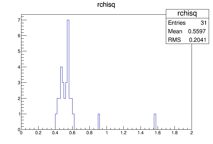
chisq/dof plot attached - I'm using TGraph to fit, which assumes errors
of 1 mV per data point. I use the time range (-200, 60).

On Thu, 3 Apr 2014, Gabriel CHARLES wrote:

> Could you both provide an average value of chi square that the different
> parametrization can be compared easily, please ?
>
> Also, from the simulation it appears that the rising edge could be present.
> In attachment you will find a picture with two plots. The top one corresponds
> to the signal after the crystal and the APD, that is the input of the
> preamplifier.
> It is obtained by the convolution of the signal of the crystal and the APD.
> The crystal response is composed of the sum of two decreasing exponential
> governed by different time constants. The APD transfert function is given by
> the bottom plot (sorry for the wrong Y axis units).
>
> There is no reason for the preamplifier to reduce the tail.
>
> I think that if there is no huge difference between the chi square it would
> be better to keep the two gaussian function.
>
> ---
> Gabriel CHARLES
> Institut de Physique Nucléaire d'Orsay
>
> On Thu, 3 Apr 2014 13:15:00 -0700 (PDT), Sho Uemura wrote:
>> I tried two more parametrizations. These are parametrizations
>> commonly used for the APV25 preamp that we use in the SVT.
>>
>> CR-RC: t*exp(-t/tp)
>> 3-pole, or CR-RC-RC: t^2*exp(-t/tp)
>>
>> 3-pole seems to fit well, I think better than the asymmetric
>> Gaussian. CR-RC seems no better than the Gaussian. Other
>> parametrizations I tried (variations on CR-RC or 3-pole using more
>> than one time constant) were degenerate with CR-RC or 3-pole, so I
>> didn't include those plots.
>>
>> Plots attached are for 3-pole function. All plots for 3-pole and
>> CR-RC, and the pyroot scripts I used, are online:
>>
>> http://www.slac.stanford.edu/~meeg/ecalpulsefit/
>>
>> I also see what you see, where there are 2 clusters in the
>> distribution of shape parameters. I chose the center of the larger
>> cluster (with the faster time constant) and refit all the events with
>> this time constant fixed; those plots are named "fit2" and as expected
>> they fit the faster pulses well and the slower pulses poorly.
>>
>> More data will help.
>>
>> I plotted the three parametrizations we have, see plot4.pdf attached.
>> If we agree that the Gaussian has an unphysical rising edge, I think
>> we should use 3-pole.
>>
>> On Tue, 1 Apr 2014, Andrea Celentano wrote:
>>
>>> Dear all,
>>> here are some results about HPS Ecal signals parametrization.
>>> I took data with the crystal placed vertically, APD gain 150, room
>>> temperature. I put a threshold ~ 20 mV to keep only big enough signals,
>>> out of the noise.
>>> I acquired data with a 2.5Gs/s oscilloscope, 1 GHz bandwidth, 50 Ohm input
>>> impedance.
>>>
>>> I used the same* configuration employed at JLab for cabling: 8m 3M cable
>>> ---> passive splitter ---> 3m lemo cable.
>>>
>>> *actually I employed an 8 meters 3M cable instead of 7m because the latter
>>> is not available here in Genova.
>>>
>>> Attached you find a postcript file with the results. (outGood.ps shows the
>>> fit results covering some parts of the signal, outGood1.ps no)
>>>
>>> - Neglect first blank page
>>> - Pages from 2 to 32 are the 31 signals I got, with superimposed the fit
>>> performed with the two-gaussians parametrization. Each chi2 fit is
>>> performed independently.
>>> Signals are in mV and ns.
>>> Note that near ~ 100 ns there is probably a reflection due to some
>>> impedance mismatch in the cables chain.
>>> However,  I am not using those points to fit. I am fitting the data in
>>> between -200 ns and +80 ns. The function is then plotted in the full time
>>> range.
>>>
>>> - Last page is a summary of the fits performed. Two 1d-histograms are the
>>> distributions of the two time constants used in the parametrization. Then
>>> I am plotting also their correlation, as well as the correlation of the
>>> rise-time (par[1]) with the signal amplitude (from the fit).
>>>
>>> I noted that the fit parameters Trise, Tfall are not distributed as two
>>> gaussians. In particular, for Trise there is an accumulation of events at
>>> ~ 5 ns and ~ 7 ns, correlated with corresponding Tfall at ~ 15 and ~20 ns.
>>> Actually, I see that, other than the amplitude, signals do not have always
>>> the same shape: look, for example, at signals n.5 and n.6 (ps pages n.5
>>> and n.6).
>>>
>>> Attached you find also the C implementation of the signal parametrization,
>>> in form of a "double fun(double *x,double  *par)" used by ROOT when
>>> fitting trough TF1.
>>> Finally, I am attaching also the raw data for the 31 signals I got, so if
>>> you're interested you can play with different signal parametrizations.
>>>
>>> I am planning to take more data these days.
>>>
>>>
>>> Bests,
>>>
>>> Andrea
>>>
>
> ########################################################################
> Use REPLY-ALL to reply to list
>
> To unsubscribe from the HPS-SOFTWARE list, click the following link:
> https://listserv.slac.stanford.edu/cgi-bin/wa?SUBED1=HPS-SOFTWARE&A=1
>

########################################################################
Use REPLY-ALL to reply to list

To unsubscribe from the HPS-SOFTWARE list, click the following link:
https://listserv.slac.stanford.edu/cgi-bin/wa?SUBED1=HPS-SOFTWARE&A=1
|


